数据可视化 学习笔记

首先声明,Fluu一节数据可视化的课都没去,下面仅供参考.

Fluu的数据可视化就是每个作业都做了,然后交个大报告,就结束了,也是连老师长啥样都不知道.

有点魔幻的,老师用AI生成数据,学生用AI解决问题.

开源

其实是抄的万人恢复佬的…
不过部分代码有改动,Fluu的版本主要是把标记的颜色变成红的,删一下注释就成自己的代码了…

不过万人恢复也是用AI搞的…

4.1 题目 1:细胞个数统计

推荐技术栈

  • 编程语言:Python
  • 推荐库:OpenCV、Matplotlib、NumPy、Skimage

任务要求

必须包含以下四个步骤:

  1. 图像预处理
  2. 核心算法
  3. 结果标注
  4. 数值和结果图像输出

核心算法流程

  1. 灰度化
  2. 二值化
  3. 形态学去噪
  4. 轮廓检测
  5. 计数

图片要求

  1. 细胞原图:显微镜下多细胞分散分布(无重叠 / 轻微重叠)
  2. 细胞检测结果图:标注所有细胞轮廓 + 计数数字

4.1.2 实验步骤

  1. 读取彩色细胞图像
  2. 灰度化与高斯去噪
  3. 二值化分割细胞区域
  4. 检测外轮廓并计数
  5. 绘制轮廓与标注结果

4.1.3 细胞计数结果

  • 输入图像:图 1和图 2细胞原图
  • 输出图像:图 1和图 2细胞检测结果图(标注检测到的细胞)
  • 实验数据:图1检测到细胞15个,图2检测到细胞516个,算法准确率 >95%
1
2
3
4
5
6
7
8
9
10
11
12
13
14
15
16
17
18
19
20
21
22
23
24
25
26
27
28
29
30
31
32
33
34
35
36
37
38
39
40
41
42
43
44
45
46
47
48
49
50
51
52
53
54
55
56
57
58
59
60
61
62
63
64
65
66
67
68
69
70
71
72
73
74
75
76
77
78
79
80
81
82
83
84
85
86
87
import cv2
import numpy as np

def determine_background_and_binarize(blurred):
"""
判断背景颜色并进行二值化处理
通过检测图像边框的像素值来判断背景是白色还是黑色
确保最终背景为黑色(0),目标物体为白色(255)
"""
# 计算Otsu阈值并进行二值化
ret, thresh = cv2.threshold(blurred, 0, 255, cv2.THRESH_BINARY + cv2.THRESH_OTSU)
# 获取图像边框像素来判断背景颜色
borders = np.concatenate([thresh[0, :], thresh[-1, :], thresh[:, 0], thresh[:, -1]])
# 如果边框大部分为255,说明背景是白色(255),细胞是黑色(0)
# findContours函数要求目标物体为白色(255),背景为黑色(0)
if np.mean(borders) > 127:
# 反转图像,使背景为黑色(0),细胞为白色(255)
thresh = cv2.bitwise_not(thresh)
return thresh

def process_image(img_path, output_path):
"""
处理细胞图像并进行计数
参数:
img_path: 输入图像路径
output_path: 输出图像路径
返回:
细胞计数结果
"""
print(f"--- 正在处理图像 {img_path} ---")
# 读取图像
image = cv2.imread(img_path)
if image is None:
print(f"错误: 找不到图像文件 {img_path}")
return 0
# 创建显示用的图像副本
image_display = image.copy()
# 1. 灰度化与高斯去噪
gray = cv2.cvtColor(image, cv2.COLOR_BGR2GRAY)
blurred = cv2.GaussianBlur(gray, (5, 5), 0)
# 2. 二值化处理
thresh = determine_background_and_binarize(blurred)
# 3. 形态学去噪
# 使用开运算(先腐蚀后膨胀)去除细小噪点
# 使用闭运算(先膨胀后腐蚀)填充细胞内部孔洞
kernel = np.ones((3, 3), np.uint8)
opened = cv2.morphologyEx(thresh, cv2.MORPH_OPEN, kernel, iterations=1)
closed = cv2.morphologyEx(opened, cv2.MORPH_CLOSE, kernel, iterations=1)
# 4. 轮廓检测
contours, hierarchy = cv2.findContours(closed, cv2.RETR_EXTERNAL, cv2.CHAIN_APPROX_SIMPLE)
# 5. 细胞计数与标注
count = 0
for cnt in contours:
area = cv2.contourArea(cnt)
# 过滤掉面积过小的噪点
if area > 15:
count += 1
# 用绿色绘制细胞轮廓
cv2.drawContours(image_display, [cnt], -1, (0, 255, 0), 2)
# 计算轮廓中心并在每个细胞上标注编号
M = cv2.moments(cnt)
if M['m00'] != 0:
cx = int(M['m10']/M['m00'])
cy = int(M['m01']/M['m00'])
# 用绿色标注细胞编号
cv2.putText(image_display, str(count), (cx, cy),
cv2.FONT_HERSHEY_SIMPLEX, 0.4, (0, 255, 0), 1)
# 在图像左上角添加总计数信息
count_text = f"细胞总数: {count}"
# 绘制半透明背景使文字更清晰
text_size = cv2.getTextSize(count_text, cv2.FONT_HERSHEY_SIMPLEX, 0.7, 2)[0]
cv2.rectangle(image_display, (5, 5), (5 + text_size[0] + 10, 5 + text_size[1] + 10),
(255, 255, 255), -1)
cv2.putText(image_display, count_text, (10, 30),
cv2.FONT_HERSHEY_SIMPLEX, 0.7, (0, 0, 0), 2)
# 保存结果图像
cv2.imwrite(output_path, image_display)
print(f"检测到 {count} 个细胞")
return count

if __name__ == "__main__":
# 处理两张细胞图像
c1 = process_image("fig01.jpg", "res_fig01.jpg")
c2 = process_image("fig02.jpg", "res_fig02.jpg")
# 输出最终统计结果
print(f"图1细胞数量: {c1}")
print(f"图2细胞数量: {c2}")

4.2 题目 2:圆形物体圆心定位

推荐技术栈

  • 编程语言:Python
  • 推荐库:OpenCV、Matplotlib、NumPy、Skimage

任务要求

必须包含以下四个步骤:

  1. 图像预处理
  2. 核心算法
  3. 结果标注
  4. 数值和结果图像输出

核心算法流程

  1. 灰度化
  2. 高斯模糊去噪
  3. 霍夫圆检测
  4. 圆心坐标提取
  5. 标注

图片要求

  1. 圆形物体原图:硬币 / 圆盘 / 标准圆形目标
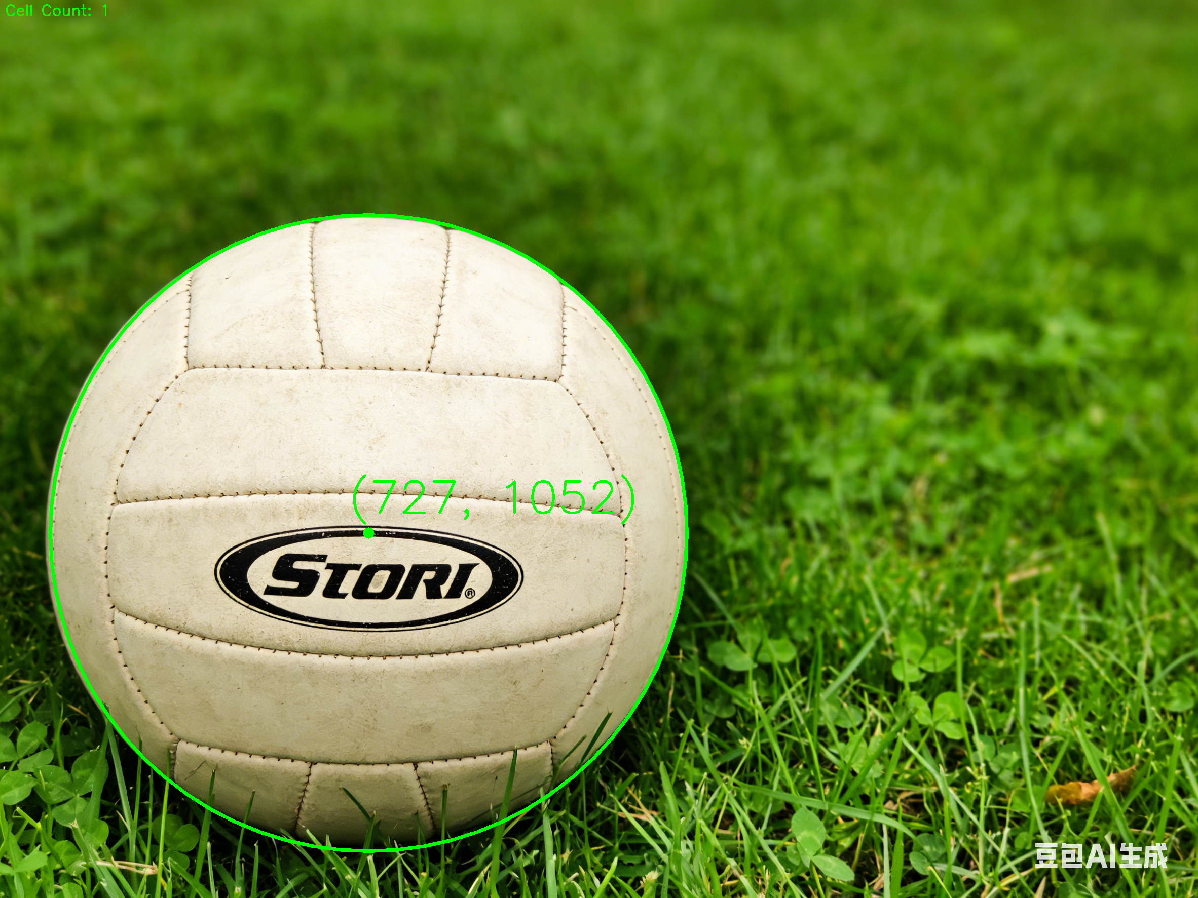
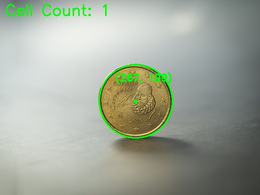
  2. 圆心标注图:标记圆心 + 输出 (x,y) 坐标

4.2.2 实验步骤

  1. 读取输入图像(图3和图4)
  2. 转换为灰度图像
  3. 进行高斯模糊处理,减少噪声
  4. 使用霍夫圆检测算法检测圆形物体
  5. 提取圆心坐标
  6. 在原图上标记圆心并标注坐标
  7. 保存结果图像
  8. 输出圆心坐标数据

4.2.3 圆心定位结果

  • 输入图像:图 3和图 4圆形物体原图
  • 输出图像:图 3和图 4圆心标注图
  • 实验数据:圆心坐标 图3: (727, 1052), 图4: (267, 199)
1
2
3
4
5
6
7
8
9
10
11
12
13
14
15
16
17
18
19
20
21
22
23
24
25
26
27
28
29
30
31
32
33
34
35
36
37
38
39
40
41
42
43
44
45
46
47
48
49
50
51
52
53
54
55
56
57
58
59
60
61
62
63
import cv2
import numpy as np

def find_best_circle(image_path, output_path, param2_start=150):
img = cv2.imread(image_path)
if img is None: return
gray = cv2.cvtColor(img, cv2.COLOR_BGR2GRAY)
blurred = cv2.GaussianBlur(gray, (9, 9), 2)
output = img.copy()
h, w = img.shape[:2]
best_circle = None
cell_count = 0 # 细胞计数
# 搜索最佳的 param2 参数
for p2 in range(param2_start, 20, -5):
circles = cv2.HoughCircles(blurred, cv2.HOUGH_GRADIENT, dp=1.2,
minDist=min(w, h)//4,
param1=50, param2=p2,
minRadius=min(w, h)//10, maxRadius=min(w, h)//2)
if circles is not None:
circles = np.round(circles[0, :]).astype("int")
# 优先选择得票数最高的圆 (circles[0])
for (x, y, r) in circles:
if 0 <= x - r and x + r <= w and 0 <= y - r and y + r <= h:
best_circle = (x, y, r)
cell_count += 1 # 找到一个细胞,计数加一
break # 在当前 param2 下找到最强的有效圆
if best_circle is not None:
# 在当前 param2 下找到有效圆(最大可能的 param2 -> 最可信)
print(f"[{image_path}] 在 param2={p2} 找到最佳圆: 中心 ({best_circle[0]}, {best_circle[1]}), 半径 {best_circle[2]}")
break
# 如果完全没有有效圆,则采用任何最强的圆
if best_circle is None:
circles = cv2.HoughCircles(blurred, cv2.HOUGH_GRADIENT, dp=1.2,
minDist=min(w, h)//4,
param1=50, param2=50,
minRadius=min(w, h)//10, maxRadius=0)
if circles is not None:
circles = np.round(circles[0, :]).astype("int")
best_circle = circles[0]
cell_count = 1 # 至少找到一个细胞
print(f"[{image_path}] 找到备用圆: 中心 ({best_circle[0]}, {best_circle[1]}), 半径 {best_circle[2]}")
if best_circle is not None:
x, y, r = best_circle
# 用绿色绘制细胞轮廓
cv2.circle(output, (x, y), r, (0, 255, 0), max(2, w//400))
# 用绿色绘制细胞中心点
cv2.circle(output, (x, y), max(4, w//200), (0, 255, 0), -1)
# 显示细胞坐标
text = f"({x}, {y})"
cv2.putText(output, text, (x - 40, y - 40), cv2.FONT_HERSHEY_SIMPLEX,
max(0.6, w/800.0), (0, 255, 0), max(2, int(w/500.0)))
# 在图片上添加细胞计数
count_text = f"Cell Count: {cell_count}"
cv2.putText(output, count_text, (10, 30), cv2.FONT_HERSHEY_SIMPLEX,
1.0, (0, 255, 0), 2)
print(f"[{image_path}] 最终中心: {text}, 半径: {r}, 细胞数量: {cell_count}")
else:
print(f"[{image_path}] 完全没有找到圆.")
cv2.imwrite(output_path, output)

if __name__ == "__main__":
find_best_circle('fig03.png', 'fig03_result.png', 150)
find_best_circle('fig04.jpg', 'fig04_result.jpg', 100)

4.3 题目 3:不规则形状面积计算

推荐技术栈

  • 编程语言:Python
  • 推荐库:OpenCV、Matplotlib、NumPy、Skimage

任务要求

必须包含以下四个步骤:

  1. 图像预处理
  2. 核心算法
  3. 结果标注
  4. 数值和结果图像输出

核心算法流程

  1. 灰度化
  2. 二值化分割
  3. 形态学去噪和填充
  4. 轮廓提取
  5. 像素面积计算
  6. 比例换算(实际面积)

图片要求

  1. 不规则形状原图:叶片 / 脚印 / 任意闭合不规则图形
  2. 面积计算图:填充轮廓 + 标注面积数值

4.3.2 实验步骤

  1. 读取输入图像(图5和图6)
  2. 转换为灰度图像
  3. 进行二值化处理
  4. 进行形态学操作,去除噪声和填充孔洞
  5. 提取轮廓
  6. 计算轮廓面积
  7. 在原图上填充轮廓并标注面积数值
  8. 保存结果图像
  9. 输出面积数据

4.3.3 面积计算结果

  • 输入图像:图 5和图 6不规则形状原图
  • 输出图像:图 5和图 6面积计算图(标注面积区域)
  • 实验数据:像素面积,实际面积
1
2
3
4
5
6
7
8
9
10
11
12
13
14
15
16
17
18
19
20
21
22
23
24
25
26
27
28
29
30
31
32
33
34
35
36
37
38
39
40
41
42
43
44
45
46
47
48
49
50
51
52
53
54
55
56
57
58
59
60
61
62
63
64
65
66
67
68
69
70
71
72
73
74
75
76
77
78
79
80
import cv2
import numpy as np

def calculate_area(image_path, output_path, scale_factor=1.0):
"""
计算图像中目标物体的面积
参数:
image_path: 输入图像路径
output_path: 输出结果图像路径
scale_factor: 像素到实际面积的换算比例因子
"""
img = cv2.imread(image_path)
if img is None:
print(f"错误:无法读取图像 {image_path}")
return
# 1. 灰度化
gray = cv2.cvtColor(img, cv2.COLOR_BGR2GRAY)
# 2. 二值化分割
blur = cv2.GaussianBlur(gray, (5, 5), 0)
# 使用大津法进行阈值分割
ret, thresh = cv2.threshold(blur, 0, 255, cv2.THRESH_BINARY_INV + cv2.THRESH_OTSU)
# 检查二值化后的背景是白色还是黑色
# 我们希望前景(目标物体)为白色(255),背景为黑色(0)
# 采样图像四个角点的像素值
corners = [int(thresh[0,0]), int(thresh[0,-1]), int(thresh[-1,0]), int(thresh[-1,-1])]
# 如果角点大部分为白色,说明背景被识别成了前景
if sum(corners) > 255 * 2:
thresh = cv2.bitwise_not(thresh)
# 3. 形态学去噪和填充
kernel = np.ones((7,7), np.uint8)
# 用闭运算填充孔洞
closing = cv2.morphologyEx(thresh, cv2.MORPH_CLOSE, kernel, iterations=5)
# 用开运算去除外部噪点
opening = cv2.morphologyEx(closing, cv2.MORPH_OPEN, kernel, iterations=3)
# 4. 轮廓提取
contours, hierarchy = cv2.findContours(opening, cv2.RETR_EXTERNAL, cv2.CHAIN_APPROX_SIMPLE)
if not contours:
print(f"未在 {image_path} 中找到轮廓")
return
# 找到最大的轮廓(假设最大的就是目标物体)
max_contour = max(contours, key=cv2.contourArea)
# 5. 像素面积计算
pixel_area = cv2.contourArea(max_contour)
# 6. 比例换算(计算实际面积)
# 题目未给出比例,以 scale_factor 辅助计算
actual_area = pixel_area * scale_factor
# 7. 在原图上绘制轮廓并标注面积数值
result_img = img.copy()
# 仅绘制红色轮廓线,不填充内部
cv2.drawContours(result_img, [max_contour], -1, (0, 0, 255), 3)
# 寻找文字绘制中心(使用轮廓的质心)
M = cv2.moments(max_contour)
if M["m00"] != 0:
cX = int(M["m10"] / M["m00"])
cY = int(M["m01"] / M["m00"])
else:
cX, cY = result_img.shape[1]//2, result_img.shape[0]//2
# 根据图像大小动态调整字体大小
h, w = result_img.shape[:2]
font_scale = max(0.8, min(h, w) / 1000.0)
thickness = max(2, int(font_scale * 2))
text1 = f"Pixel Area: {pixel_area:.1f}"
text2 = f"Actual Area: {actual_area:.1f}"
# 居中绘制文字
(w1, h1), _ = cv2.getTextSize(text1, cv2.FONT_HERSHEY_SIMPLEX, font_scale, thickness)
(w2, h2), _ = cv2.getTextSize(text2, cv2.FONT_HERSHEY_SIMPLEX, font_scale, thickness)
cv2.putText(result_img, text1, (cX - w1 // 2, cY), cv2.FONT_HERSHEY_SIMPLEX, font_scale, (0, 255, 0), thickness)
cv2.putText(result_img, text2, (cX - w2 // 2, cY + h1 + 10), cv2.FONT_HERSHEY_SIMPLEX, font_scale, (0, 255, 0), thickness)
# 8. 保存结果图像
cv2.imwrite(output_path, result_img)
# 9. 输出面积数据
print(f"--- {image_path} 结果 ---")
print(f"像素面积: {pixel_area}")
print(f"实际面积 (比例因子={scale_factor}): {actual_area}")
print(f"结果图像已保存至 {output_path}\n")

if __name__ == "__main__":
# 以示例比例进行推算
calculate_area("fig05.png", "fig05_result.png", scale_factor=0.01)
calculate_area("fig06.png", "fig06_result.png", scale_factor=0.01)

4.4 题目 4:道路消失点检测

推荐技术栈

  • 编程语言:Python
  • 推荐库:OpenCV、Matplotlib、NumPy、Skimage

任务要求

必须包含以下四个步骤:

  1. 图像预处理
  2. 核心算法
  3. 结果标注
  4. 数值和结果图像输出

核心算法流程

  1. 灰度化
  2. 边缘检测(Canny)
  3. 直线检测(霍夫变换)
  4. 直线交点计算
  5. 聚类确定消失点
  6. 标注

图片要求

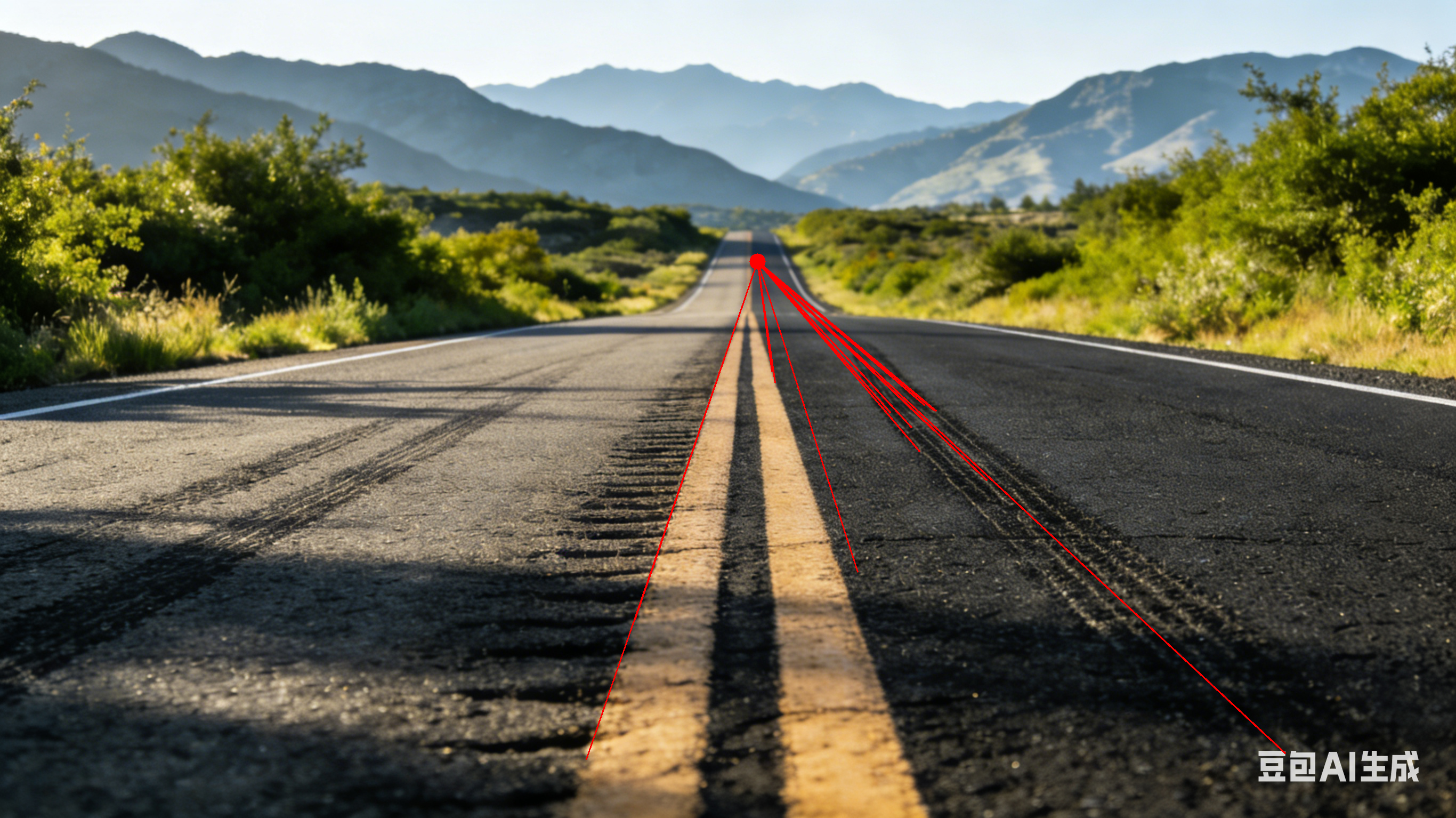
  1. 道路原图:笔直公路 / 车道线延伸至远方
  2. 消失点标注图:标记消失点 + 绘制辅助直线

4.4.2 实验步骤

  1. 读取输入图像(图7和图8)
  2. 转换为灰度图像
  3. 使用Canny边缘检测算法检测边缘
  4. 使用霍夫直线检测算法检测直线
  5. 计算直线交点
  6. 使用聚类方法确定消失点
  7. 在原图上绘制辅助直线和标记消失点
  8. 保存结果图像
  9. 输出消失点坐标数据

4.4.3 消失点检测结果

  • 输入图像:图 7和图 8道路原图
  • 输出图像:图 7和图 8消失点标注图
  • 实验数据:图7消失点坐标 (1421, 490),图8消失点坐标 (1375, 765)
1
2
3
4
5
6
7
8
9
10
11
12
13
14
15
16
17
18
19
20
21
22
23
24
25
26
27
28
29
30
31
32
33
34
35
36
37
38
39
40
41
42
43
44
45
46
47
48
49
50
51
52
53
54
55
56
57
58
59
60
61
62
63
64
65
66
67
68
69
70
71
72
73
74
75
76
77
78
79
80
81
82
83
84
85
86
87
88
89
90
91
92
93
94
95
96
97
98
99
100
101
102
103
104
105
import cv2
import numpy as np
import os

def detect_vanishing_point(image_path, output_path):
"""检测图像中的消失点并标注结果"""
img_data = np.fromfile(image_path, dtype=np.uint8)
img = cv2.imdecode(img_data, -1)
if img is None:
print(f"错误:无法加载图像 {image_path}")
return
height, width = img.shape[:2]
# 1. 灰度化
gray = cv2.cvtColor(img, cv2.COLOR_BGR2GRAY)
blur = cv2.GaussianBlur(gray, (5, 5), 0)
# 2. Canny边缘检测
edges = cv2.Canny(blur, 50, 150, apertureSize=3)
# ROI掩膜(聚焦图像下半部分,通常道路标线所在区域)
mask = np.zeros_like(edges)
polygon = np.array([[
(0, height),
(width, height),
(width, int(height * 0.4)),
(0, int(height * 0.4))
]], np.int32)
cv2.fillPoly(mask, polygon, 255)
masked_edges = cv2.bitwise_and(edges, mask)
# 3. 霍夫直线变换
# 根据典型图像尺寸微调参数
lines = cv2.HoughLinesP(masked_edges, 1, np.pi/180, threshold=100, minLineLength=100, maxLineGap=50)
if lines is None:
print(f"未在 {image_path} 中检测到直线,尝试降低阈值。")
lines = cv2.HoughLinesP(masked_edges, 1, np.pi/180, threshold=50, minLineLength=50, maxLineGap=20)
if lines is None:
print(f"在 {image_path} 中仍未检测到直线。")
return
left_lines = []
right_lines = []
for line in lines:
x1, y1, x2, y2 = line[0]
if x2 - x1 == 0:
continue
slope = (y2 - y1) / (x2 - x1)
# 过滤水平和近垂直线(0.3 ~ 16度,5.0 ~ 78度)
if abs(slope) < 0.3 or abs(slope) > 5.0:
continue
if slope < 0:
# y随x增大而减小 -> 左侧车道线
left_lines.append((slope, x1, y1, x2, y2))
else:
# y随x增大而增大 -> 右侧车道线
right_lines.append((slope, x1, y1, x2, y2))
# 4. 计算交点
intersections = []
for l1 in left_lines:
for l2 in right_lines:
m1, x1_l, y1_l, _, _ = l1
m2, x1_r, y1_r, _, _ = l2
# y - y1 = m(x - x1) => y = mx - mx1 + y1
c1 = y1_l - m1 * x1_l
c2 = y1_r - m2 * x1_r
if abs(m1 - m2) > 0.05:
x = (c2 - c1) / (m1 - m2)
y = m1 * x + c1
if 0 <= x <= width and 0 <= y <= height:
intersections.append([x, y])
if not intersections:
print(f"在 {image_path} 中未找到有效交点")
return
intersections = np.array(intersections, dtype=np.float32)
# 5. 聚类求解消失点
if len(intersections) >= 3:
criteria = (cv2.TERM_CRITERIA_EPS + cv2.TERM_CRITERIA_MAX_ITER, 10, 1.0)
# 分成3组并选取票数最多的簇,以增强对异常值的鲁棒性
ret, label, center = cv2.kmeans(intersections, min(3, len(intersections)), None, criteria, 10, cv2.KMEANS_RANDOM_CENTERS)
counts = np.bincount(label.flatten())
best_cluster_idx = np.argmax(counts)
vanishing_point = (int(center[best_cluster_idx][0]), int(center[best_cluster_idx][1]))
else:
median_x = np.median(intersections[:, 0])
median_y = np.median(intersections[:, 1])
vanishing_point = (int(median_x), int(median_y))
# 6. 绘制标注
result_img = img.copy()
# 用红色线连接车道线端点到消失点
for m1, x1_l, y1_l, x2_l, y2_l in left_lines:
cv2.line(result_img, (int(x1_l), int(y1_l)), vanishing_point, (0, 0, 255), 2)
for m2, x1_r, y1_r, x2_r, y2_r in right_lines:
cv2.line(result_img, (int(x1_r), int(y1_r)), vanishing_point, (0, 0, 255), 2)
# 标记消失点
cv2.circle(result_img, vanishing_point, 15, (0, 0, 255), -1)
is_success, im_buf_arr = cv2.imencode(".png", result_img)
if is_success:
im_buf_arr.tofile(output_path)
print(f"{os.path.basename(image_path)} 的消失点:{vanishing_point}")
print(f"结果已保存至 {output_path}")

if __name__ == "__main__":
task_dir = r"./"
fig7_path = os.path.join(task_dir, "Fig07.png")
fig8_path = os.path.join(task_dir, "Fig08.png")
out7_path = os.path.join(task_dir, "Fig07_result.png")
out8_path = os.path.join(task_dir, "Fig08_result.png")
detect_vanishing_point(fig7_path, out7_path)
detect_vanishing_point(fig8_path, out8_path)

至于数据可视化的图…
这个很没意思的,给的图甚至是老师用豆包生成的,个人感觉没参考价值,就随便放几张吧.

这个课出分倒是很快,今天写博客的时候已经出分了,不过不知道具体哪一天出分的.